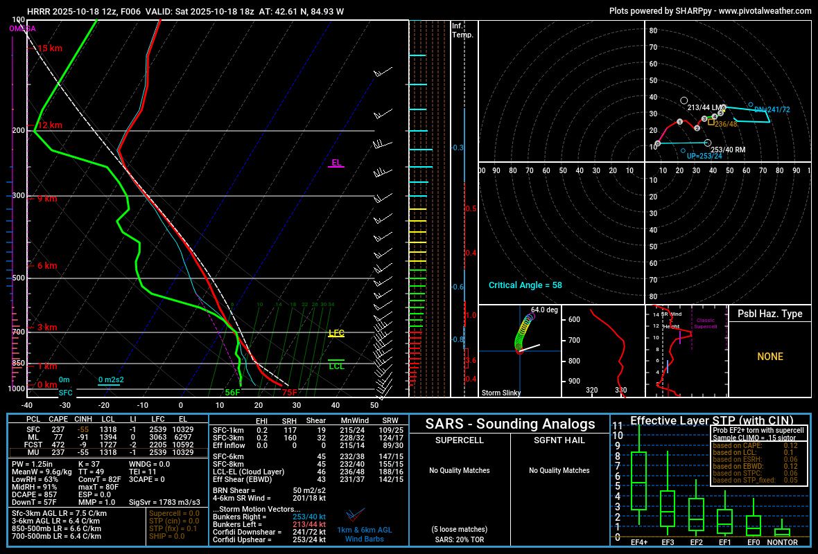
How to Read Soundings

Soundings summarize temperature, moisture, and wind with height. This page is a compact reference for reading the main features on a Skew‑T and hodograph.

Skew‑T anatomy

This is a Skew-T graph:

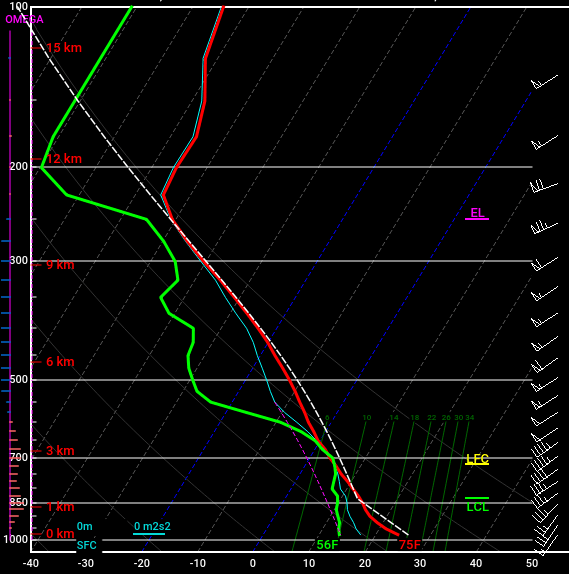
• Vertical axis: pressure in mb (1000 near the surface → 100 at the top). Higher on the chart = higher in the atmosphere.
• Temperature lines: slanted up‑right. Red line = environmental temperature; green line = environmental dewpoint.
• Parcel trace (often dashed): how a surface or mixed parcel would warm/cool if lifted. Dry‑adiabatic to the LCL, moist‑adiabatic above.
• Background guides: brown straight lines (dry adiabats), blue curved lines (moist adiabats), and diagonal green mixing‑ratio lines (constant water vapor).

Key levels & what they imply

• LCL — cloud base of a lifted parcel
  Plain: Lower LCLs mean lower cloud bases — easier for stretching and tornado potential. Target: <~1.2 km AGL.
  Detail: Backed surface winds that raise moisture depth can drop LCL and boost 0–1 km SRH ingestion.
• LFC — start of free ascent
  Plain: If the LFC is very high (>~2 km), storms start high and look ‘stilted’ — more wind/hail, fewer tornadoes.
  Detail: Watch the heating needed to lift parcels to their LFC; 1–3 °C shortfall is close, 5–7 °C is a reach without strong forcing.
• EL — buoyancy top
  Plain: Higher EL → taller storms and usually more lightning.
  Detail: EL temperature relative to −20 to −30 °C matters for charge separation and hail growth depth.
• CAPE (SBCAPE/MLCAPE/MUCAPE)
  Plain: More CAPE = stronger updraft potential, but only if parcels can reach it.
  Detail: Use MLCAPE (100–150 mb mixed) for surface‑based setups; MUCAPE governs elevated storms above a cap.
• CIN (the cap)
  Plain: Some cap is good — it keeps junk from firing early. Too much cap and nothing initiates.
  Rules of thumb: 25–75 J/kg focuses storms; 100–150+ J/kg needs strong lift or late‑day heating.

Lapse rates, EML, and why hail explodes (or not)

• Mid‑level lapse rate (700–500 mb): 7–9 °C/km favors big updraft speeds and hail; ≤6 °C/km fights severe growth.
• Low‑level lapse rate (sfc–3 km): Steepening during afternoon = deeper mixing, stronger gusts, faster cap erosion.
• EML: A warm, dry layer around 700–800 mb that caps convection. If surface moisture is deep and lift arrives, storms can go from nothing to explosive quickly.

Downdrafts & hail signals

• DCAPE: Bigger DCAPE → stronger downburst potential, especially with an inverted‑V near the surface.
• Freezing/−10/−20 °C levels: Lower heights plus steep mid‑level lapse rates = larger hail. CAPE through the −10 to −30 °C layer is the hail fuel.

Hodograph 101 (shape → storm behavior)

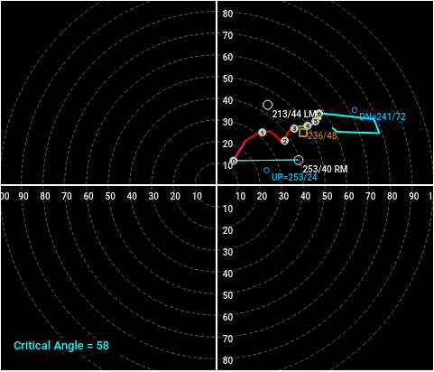
The hodograph plots wind with height, tail at the surface, head aloft. Read its length (speed shear) and curvature (directional shear).

• 0–6 km bulk shear: ~20–25 kt → multicells; ~35–45 kt → supercells likely; >50 kt → robust organization (lines if forcing is strong).
• 0–1 km shear: ≥20 kt helps mesocyclones; ≥30–40 kt with curvature raises tornado potential.
• SRH (0–1/0–3 km): Streamwise vorticity available to the storm. ≥150 m²/s² (0–1 km) supportive; ≥250–300 m²/s² concerning when LCLs are low and CIN modest.
• Critical angle: Angle between storm‑relative inflow and the 0–500 m shear vector. ~60–90° commonly appears in tornadic setups; tiny angles can starve storms of streamwise vorticity.
• Effective shear / effective inflow layer: Uses only the buoyant layer. Effective bulk shear ≥25–30 kt is a strong supercell signal even if surface‑based depth is shallow.

Putting it together: fast decision rules

• Tornadic supercell window: MLCAPE 1000–3000 J/kg, low LCLs, modest CIN, 0–1 km SRH ≥150–250 m²/s², 0–6 km shear ≥35–45 kt, curved hodograph, and a boundary that locally backs surface winds.
• Significant hail: Steep 700–500 mb lapse rates (≥7.5 °C/km), CAPE through −10 to −30 °C, adequate mid‑level flow, and not‑too‑high freezing level.
• Damaging wind / QLCS: Large DCAPE, deep mixed boundary layer, strong low‑mid flow aligned with forcing, straighter hodograph.

Red flags & gotchas

• Warm noses (850–700 mb) increase CIN and can melt hail; look for cooling aloft or stronger lift before committing.
• Elevated storms (MUCAPE only): great lightning/hail potential but poor tornado odds without surface rooting.
• Skinny CAPE: tall positive area but weak acceleration — lots of storms, little punch.
• Dry slots near 700 mb: encourage evaporation → stronger downdrafts; wind may dominate.

Field workflow (practical)

1. Morning: Scan multiple soundings along your corridor. Circle places with deep moisture and LCL <~1.2 km.
2. Late morning–early afternoon: Track boundaries; recheck if heating/forcing will chip away at CIN during 20–00z.
3. Pre‑initiation: Compare current obs to the sounding. If you still need +2–3 °C of heating to reach LFC, stay near focused lift or a boundary.
4. Nowcast: Favor zones where surface winds back beneath strong 850‑mb flow; verify hodograph curvature and effective shear, not just composites.
5. Post‑event: Log LCL/LFC/EL, CAPE shape, shear, storm mode, and failures. Personal analogs beat generic indices over time.

Checklist: does this sounding deserve my gas money?

• LCL below ~1.2 km AGL and moisture depth ≥100–150 mb
• MLCAPE ≥1000–1500 J/kg with fat CAPE below 3 km
• CIN small/moderate and eroding by late afternoon
• 0–6 km shear ≥35–45 kt; effective bulk shear ≥25–30 kt
• 0–1 km SRH ≥150–250 m²/s² with curved hodograph and decent critical angle
• Mid‑level lapse rate ≥7.0–7.5 °C/km (hail potential)
• No crippling warm nose; a boundary or focused lift nearby

Glossary (fast)

• LCL: Lifted Condensation Level — first cloud base of a lifted surface parcel.
• LFC: Level of Free Convection — where the lifted parcel becomes warmer than the environment.
• EL: Equilibrium Level — top of positive buoyancy region.
• CAPE/CIN: Positive/negative buoyant energy areas — updraft fuel vs. cap.
• SRH: Storm‑Relative Helicity — ingestion of streamwise vorticity.
• EML: Elevated Mixed Layer — warm/dry cap source over cooler/moister low levels.
• DCAPE: Downdraft CAPE — evaporative cool potential and gust strength proxy.

With these reads you can move beyond ‘green/red squiggles’ and evaluate initiation likelihood, storm mode, and failure risks quickly and consistently.